Fitting a polynomial to data using the singular value decomposition

When analysing data, often a good starting point is to fit a polynomial of degree \(n\) to those data. In this exercise, I demonstrate how we can approach this problem with linear algebra, in particular the singular value decomposition (SVD) of a matrix representing input data provides an algorithm to find the polynomial that fits the data. The SVD also helps with reducing overfitting and improving numerical stability.

To illustrate this our data will be

$$ \begin{align} t, \hat{f}(t) \end{align} $$

where \(t\) will be \(m\) equally spaced points along the unit interval (i.e., $t=t_1, \cdots, t_m$). For illustration, the function \(\hat{f}\) will be \(f(t) = 2 + \cos(8t) + \sin(16t)\) plus a random perturbation.

To fit an \(n\)-th order polynomial, \(P_n(t) = b_0 + b_1t + \cdots +b_nt^n\), we substitute in input output pairs \((t_i, \hat{f}_i)\), giving

$$ \begin{align*}
\hat{f}_1 &= b_0 + b_1(t_1) + \cdots + b_nt_1^n \cr &\cdots \cr \hat{f}_m &= b_0 + b_1(t_m) + \cdots + b_nt_m^n \end{align*} $$

Recognising that this is a system of linear equations we can instead describe it with the notation

$$ \begin{align} \hat{f} &= A b \end{align} $$

where \(A\) is a matrix containing the various powers of the input data (called the Vandermonde matrix), \(b\) is a vector containing the to be determined polynomial coefficients, and \(\hat{f}\) is a vector of our output data.

If \(A\) is non-singular (i.e., invertible; guaranteed for a Vandermonde matrix with unique \(t_i\)) a solution to this system exists, namely \(b = A^{-1}\hat{f}\).

There are various methods of finding the inverse of a matrix; in this instance we can use the singular value decomposition of \(A\). For real-valued matrices the singular value decomposition is a factorisation of the form

$$ \begin{align*} A = U \Sigma V^T \end{align*} $$

with the properties that \(u\) and \(v^t\) are unitary (the inverses of these matrices are their transposes), with dimensions \(m\times m\) and \(n \times n\), respectively. And \(\Sigma\) is a \(m\times n\) diagonal matrix, whose entries are descending singular values of \(A\).

Substituting this into \((2)\) gives

$$ \begin{align} \hat{f}(t) &= U \Sigma V^T b \end{align} $$

Since, inverting unitary and diagonal matrices is straightforward we now have an algorithm for solving our system of equations. First, left-multiplying \((3)\) by \(U^T\) gives

$$ \begin{align*} U^T\hat{f}(t) &= U^TU\Sigma V^T b \cr &= \Sigma V^T b \end{align*} $$

Next, left-multiply by the inverse of \(\Sigma\) which will just be itself with the diagonal entries reciprocated.

$$ \begin{align*} \Sigma^{-1} U^T \hat{f}(t) &= V^T b \end{align*} $$

Finally, left-multiply by \(V\) to get the solution

$$ \begin{align*} V\Sigma^{-1} U^T \hat{f}(t) &= b \end{align*} $$

The theory can be put to practice with the following MATLAB code (it works in Octave too, though the axes' labels don't format nicely and for large enough \(n\) Octave's svd function is not numerically stable):

clearvars

% Set m and n
m = 30-1; % 30 data points
n = 15; % degree 15 polynomial

% Compute t and f(t). From here on, single precision will be used
t = single([0:m]/m);
f = 2 + cos(8*t) + sin(16*t);
%{
To the true data add random numbers normally distributed with mean zero and variance of 0.05.
For reproducibility also specify the seed and the generator used.
https://au.mathworks.com/help/matlab/math/random-numbers-with-specific-mean-and-variance.html
%}
rng(42,'twister');
f_hat = f + sqrt(0.05).*randn(1, m+1, 'single');
f_hat_vec = f_hat'; % Transpose, so that it is a column vector

% Create A, whose i-th column is t^i
i = single([0:n]);
A = (transpose(t)).^i;

% Step 0. Compute reduced SVD using MATLAB's svd function
[U, S, V] = svd(A, 'econ');

% Step 1. Let c be the result
c = (U')*f_hat_vec;

% Step 2. Let d be the result
Sd = diag(S);
inv_Sd = 1.0./Sd;
d = inv_Sd.*c;

% Step 3. Finally find the coefficient vector b = Vd
b = V*d;

% Evaluate P_n(t) with this b
Pt = A*b;

% Plot of the data and the polynomial
figure(1)
plot(t, Pt, 'r--.')
hold on
plot(t, f, 'k--x')
plot(t, f_hat, 'b--.')
xlabel('$Inputs (t)$','Interpreter','latex')
ylabel('Outputs','Interpreter','latex')
legend('$P_{15}(t)$','$f(t)$','$\hat{f}(t)$','Interpreter','latex','Location','southeast','FontSize',14)
title('When $n=15$','Interpreter','latex')

When \(N\) is set to \(30\), the resulting polynomial overfits the perturbed data (see Figure 1 below).

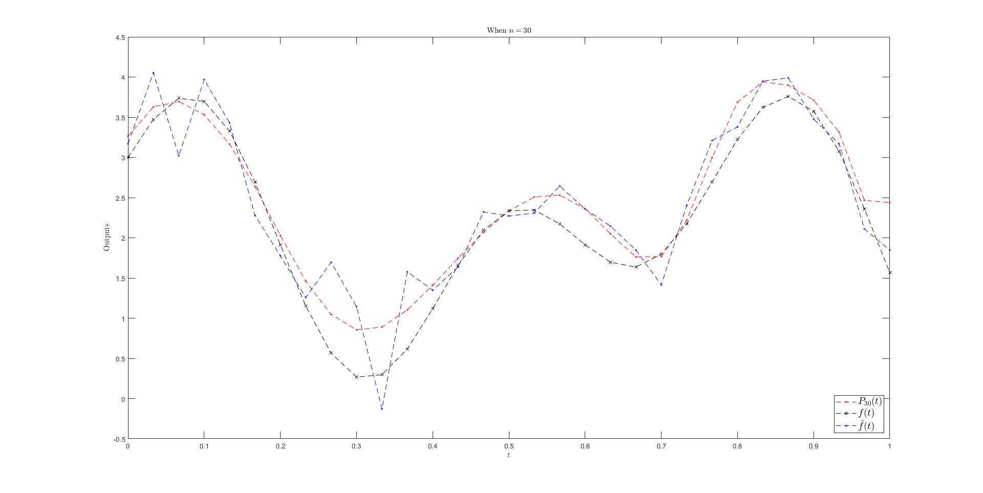Figure 1: When n=30, the polynomial overfits the noisy data

Or when run in Octave (with different random numbers) the resulting polynomial is incredibly poor (Octave's svd seems to be inaccurate in producing the last singular values).

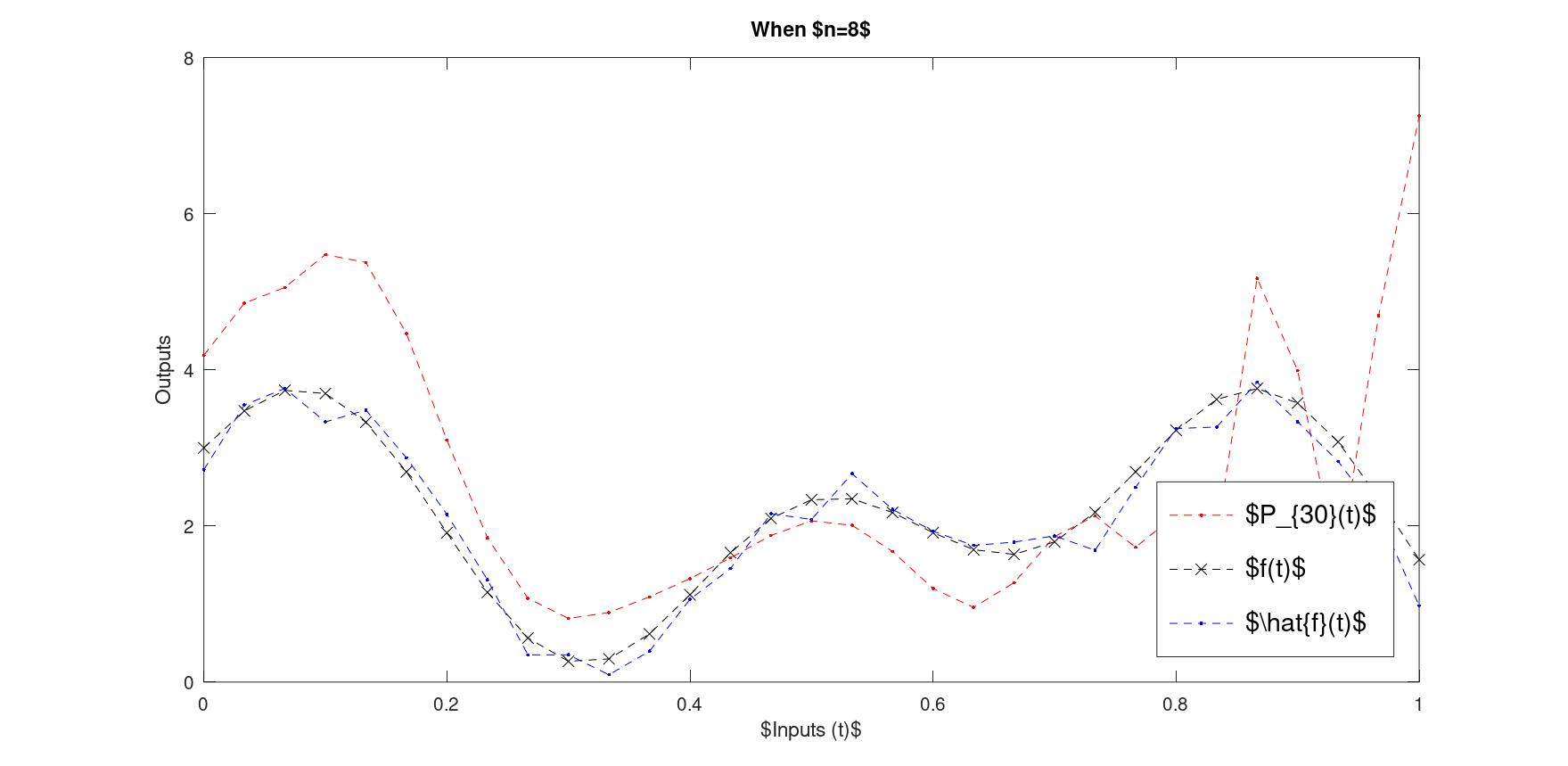Figure 2: Octave's svd function shows numerical instability

Both these issues (overfitting and numerical instability) are overcome by finding a polynomial with lower degree. We can do this by either setting \(n\) much smaller (since this specifies the polynomial degree) and re-running the script, or by setting small singular values to be zero and continuing. Before demonstrating this, a brief justification.

Consider again the SVD of \(A\), if we split \(\Sigma\) into one matrix per singular value with all other entries being zero, i.e. the \(I\)-th such matrix can be described as \(\Sigma_i = \text{diag}(0,\cdots, \sigma_i,\cdots, 0)\) then we can write

$$ \begin{align*} A &= U(\Sigma_1 + \cdots + \Sigma_n)V^T \end{align*} $$

Focusing on the first two terms, notice that a matrix times a diagonal matrix with entries of all zero except for one will return the \(I\)-th column with entries multiplied by \(\sigma_i\) with all other columns simply containing zeros. The non-zero column of each of the resulting matrices, when multiplied with \(V^T\) multiplies with the \(i\)-th row like an outer product. Allowing us to write

$$ \begin{align*} A &= \sum_{i=1}^n \sigma_i u_i v_i^T \end{align*} $$

Intuitively, for \(\sigma_i\approx 0\) the corresponding matrix in the above expression is approximately entirely comprised of zeros, hence discarding small singular values will still give a good approximation of \(A\).

Continuing with the examples. In MATLAB setting a lower \(n\) gave:

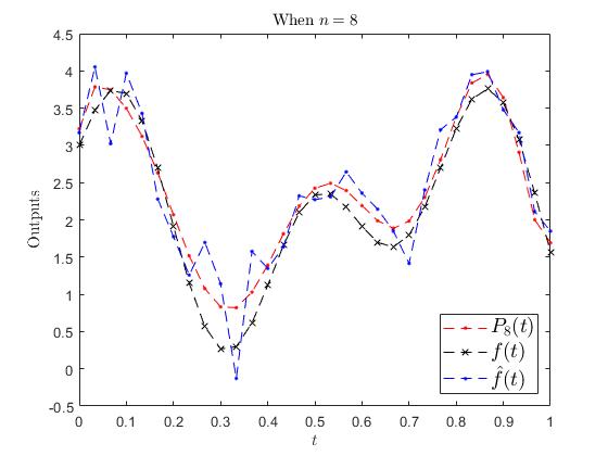Figure 3: With n=8, the fit is much better

In Octave after inverting \(\Sigma\), keeping only the first eleven singular values non-zero and continuing the script gave:

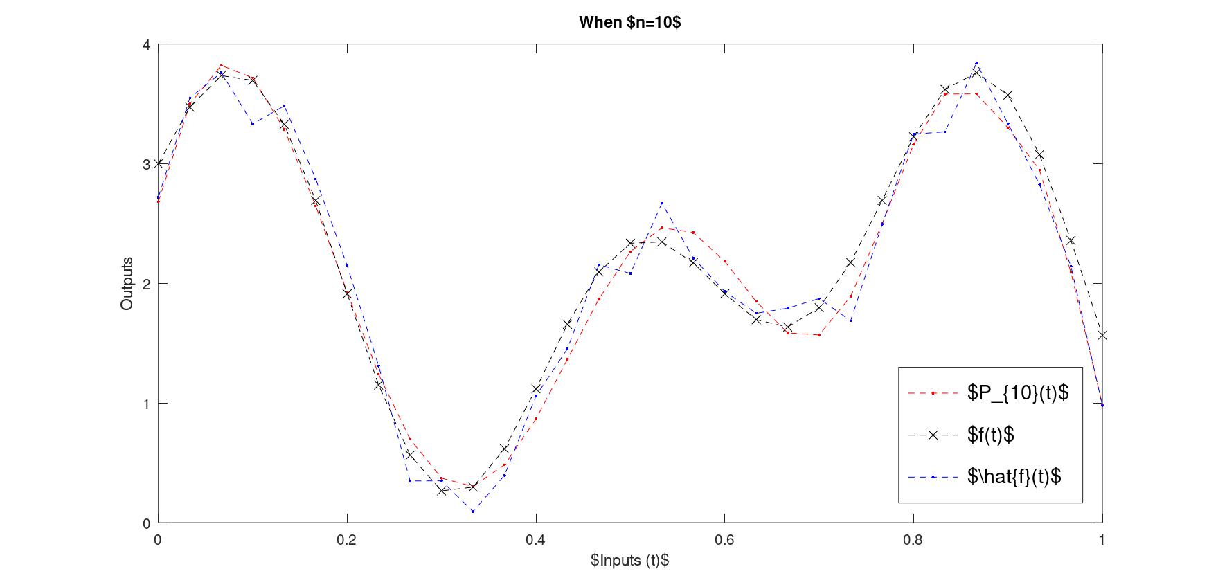Figure 4: Truncating singular values improves the fit

To measure how good the fit is in this last example, the \(2\)-norm between the polynomial and the perturbed data is 1.08, between the polynomial and the 'true' data it is similar at 1.12, both are smaller than the amount of perturbation 1.29 (as measured by the \(2\)-norm again).